Disruptive Technology Assessment Game

This article led our internal electronic news service for Defence R&D Canada, but since it is internal and not generally available outside our intranet I thought I would post it as an example of an activity I recently did at work.  (For those who can't tell, I am the guy with the blue shirt in the middle of the photo.)

Pictured here are military officers from CFB Suffield and DRDC Suffield, along with scientific personnel who participated in the inaugural Disruptive Technology Assessment Game (DTAG) held on March 3 and 10, 2010. This adapted-for-Canada, two part war game was the first of its kind which brought the Canadian Forces and defence scientists together to identify and assess the disruptive potential of technologies.

Defence scientists may spend weeks, months, and sometimes years exploring technologies that can give the Canadian Forces an advantage. A common question lingers, "how can we be sure this technology can deliver in reality what the CF needs to be ahead of the curve?" This quandary can be a source of consternation for both scientists and military personnel alike - particularly as it relates to disruptive technologies which give the military an operational advantage and competitive edge over adversaries.

As a solution to this complex issue, a Disruptive Technology Assessment Game (DTAG) was organized at DRDC Suffield on March 3 and 10, 2010 by Dr. Gitanjali Adlakha-Hutcheon while on assignment at Suffield from the Office of Chief Scientist, DRDC.

"DTAG serves as a tool for red-teaming using a mock scenario where blue and red teams square off. Each team is armed with futuristic technologies which are depicted by playing cards called Idea of Systems (IoS)," explains Dr. Adlakha-Hutcheon the DTAG organizer and chair. She elaborates, "Playing out these cards enables DRDC and the CF to play the Devil's advocate and evaluate the strengths and weakness of new technologies within military concepts of operations."

The Suffield DTAG was divided into two parts. Part One was designed to identify the IoS cards (technologies) expected to have the potential to disrupt the blue or red team's concept of operations (CONOPs). Part Two took place a week later using the traditional NATO DTAG style to play out the IoS cards to assess their disruptive abilities.

Part One - March 3: Two purple teams comprised of defence scientists and engineers came together for a structured brainstorming session. In a race against the clock the teams produced IoS cards to support a blue team mission. A panel of judges then decided which cards could pose the red team with the greatest number of rebuttals. During this exercise these IoS cards were challenged by military officers who red-teamed (a military term for acting as a challenge function) the exercise. After a rigorous challenge, four cards were finally selected to be played out for DTAG, Part Two.

Part Two - March 10: Eight military officers from CFB Suffield and DRDC Suffield, along with two scientific advisors were divided into a red team and a blue team. Executed over four sessions, this game used a single vignette made up of several asymmetric elements. In session one each team developed a CONOPs. The red team and blue team then faced-off in session two for a military confrontation chaired by LCol Dan Drew, Senior Military Officer, DRDC Suffield. In session three the IoS cards were introduced, forcing both teams to re-focus their CONOPs. The fourth session, was the battle royal with a technology-led confrontation between the two teams which was chaired by Dr. Scott Duncan, DRDC Suffield.

Participants really got into the game and the results reflected this commitment. Part One was valuable as it brought awareness among S&T professionals for DTAG as a tool for structured red-teaming. Part Two clearly identified technological systems requiring further exploration by DRDC in its role as trusted advisor and risk mitigator to optimize the benefits for the CF. The DTAG was formally wrapped up with a report to DG, DRDC Suffield.

Original Article:  Leo Online 19 March 2010

 

A Sense of Perspective - Astronomically Speaking

Astronomical scales are something that is frankly beyond human comprehension.  Sure, we can calculate sizes and distances and map things against each other and we may feel that we have a metric of the scales involved - but this is simply academic/scientific knowledge - not internalized understanding.  Real comprehension in this case becomes almost transcendental.  This set of images, (source unfortunately unknown - I received them in an email...), which shows the relative scales of the familiar planets and a few familiar stars from our local neighborhood helps to make this point in a very graphic way:

First we have the terrestrial planets, of which Earth is the largest, and we also include Pluto as a representative member of the Kuiper Belt Objects.  There are many thousands (almost certainly more than 100,000) of these Pluto-type objects - some even larger than Pluto - in a broad torus that rings the Sun from the orbit of Neptune out to about 55 Astronomical Units (AU). (1AU is the average distance from the Sun to the Earth.)

Here we add the aptly named "Gas Giant" planets - Jupiter, Saturn, Uranus, and Neptune.

All of the planets are dwarfed by the Sun.

The Sun is a member of the main sequence "Dwarf" stars, and has a spectral classification of G2V.  This means that it is a yellow star, about 20% towards being an orange star, on the main sequence. Between 7-8% of all main sequence stars are G.  Sirius is the brightest star in the sky, as seen from Earth.  Pollux and Arcturus are familiar stars, easily visible from Earth.

But even these large stars are utterly dwarfed by "Red Giant" stars like Aldebaran, Betelgeuse and Antares.  As the Sun nears the end of its life, it will also grow into a red giant star like these.

So far we have just been talking about planets and stars.  Stars are only as "motes of dust" in the "dust storms" that are Galaxies!  (Only less so; the relative distances between grains of dust in a dust storm are orders of magnitude closer than the relative distances between stars in a galaxy.)

Credit: R. Williams (STScI), the Hubble Deep Field Team and NASA
Original image available here: http://hubblesite.org/newscenter/archive/1996/01/image/e
 

Here is where things get really "transcendental". In 1995 the Hubble Space Telescope was pointed at an "empty" region of the sky in the "Big Dipper", and captured this image.  If you imagine a pin held at arms length, the head of the pin would cover the area of the sky that is about the size of this image. Scientists have counted more than 3000 galaxies in this image.  (There are only a few foreground stars , which can be identified by their "spikes".)  It would take more than 500,000 images like this to cover the whole sky. If we did this, we might expect to see about 1,500,000,000 (one and one half billion) galaxies. The Milky Way is a fairly typical galaxy.  There are more than 100,000,000,000 (one hundred billion) stars in the Milky Way galaxy alone.

And now we have this new image, known as the Hubble Ultra Deep Field 2009 (HUDF09), which was taken by the Wide Field Camera 3 in August 2009. The faintest and reddest objects in the image are the oldest galaxies ever identified.  The photons that were captured from these ancient galaxies were emitted some 600 million to 900 million years after the Big Bang and have been traveling through space - at the speed of light - for about 13 billion years in order to reach us.

I think that it has to be very hard to maintain a conceit about mankind's central importance to the universe when faced with this kind of data.

Existential Genealogy?

While reviewing the science news for the day I came across an intriguing article (really!) describing a study by Professor Carla Almeida Santos and her graduate student Grace Yan entitled "Genealogical Tourism: A Phenomenological Examination" (Journal of Travel Research 2010; 49; 56 originally published online 24 February 2009; DOI: 10.1177/0047287509332308). While the article itself is quite learned (and a bit inaccessible for the uninitiated) I found some of the interpretations of their work by the authors themselves to be quite insightful and in good agreement with my own existential experiences and feelings as an amateur genealogist.

A few worthwhile quotes from the authors press release describing their work:

"Genealogical tourism provides an irreplaceable dimension of material reality that's missing from our postmodern society," Santos said.

"Traveling to the old church where one's great grandparents used to worship in rural Ireland, or buying a loaf of bread from a tiny grocery store in the village where one's grandmother was from in Greece create a critical space to imagine and feel life as a form of continuation," says co-author and U. of I. graduate student Grace Yan.

"Genealogical tourism capitalizes on this (a world where mediated, inauthentic experiences have become such an ingrained part of everyday life that we're almost unaware of it) by allowing individuals to experience the sensuous charms of antiquity, and provides a way of experiencing something eternal and authentic that transcends the present," Santos said.

"According to our research, the baby boomer generation now constitutes the primary profile of genealogical travelers," Yan said. "Aging plays an important role in defining a person's choice of tourism, and genealogical travel is contemporary society's way of attaining a more coherent and continuous, albeit imagined, view of ourselves in connection with the past."

"Diaspora definitely plays an important role in popularizing genealogical tourism," Santos said. "Individual cultural and ethnic identities exist in fragmented and discontinuous forms in the U.S. Traveling to identify with an unknown past seems to give existence to meanings and values that the individual then carries forward on into their present."

Since diaspora is a ubiquitous condition in our multicultural country, "our ancestors' past seems less retrievable and almost mythical," Yan said.

"A lot of us may feel that there's a tension between the need to feel connected and the need to be individualistic," Santos said. "Genealogical travel gives us a practical way to explore those feelings and move toward a deeper understanding of our identities."

"Not only does it help to mitigate the desires and anxieties about our age, genealogical tourism also encourages us to take a more humanistic approach toward issues of belonging, home, heritage and identity," she said.

Using AviStack to Create a Lunar Landscape - Part 2

AviStack Noob

So now I had the AviStack software installed, and (finally!) a selection of .avi format video files that it could read.  It was time to dive into the program!

 

Figure 1 - The Empty AviStack Workspace

On starting the program the user is presented with an empty workspace (Figure 1).

The File menu item is used to get input files for the program to work with.  These inputs can be an individual movie - preferably .avi (Load Movie), individually selected images (Load Images), or automatically selected sets of all images in a specific folders (Load Folder).  In addition, it is possible to use the File menu to save "AviStack Data" files (.asd) that represent the state of data processing at a user save point (Save Data) so that by reloading the data file (Load Data) AviStack can resume processing where it left off.  This is useful if you have to interrupt your work for a while, and don't want to lose the work you have already done.  Also, to use the batch functionality you will need to have progressed through the work-flow to the point of having created the reference points (the "Set R Points" button) or beyond, and then save the .asd file for each movie or image set you want to batch process.  Then, when you are ready to run your set of sub-projects through the batch function you will load all of the relevant .asd files and start the batch.

The Settings menu item lets you manage the default settings for the sliders and radio buttons (Default Settings), manage optical "flat fields) (Flat-Field), manage "dark frames" (Dark Frame), and change language and font preferences.  Default settings are useful if you have different preferences for different types of projects; for example lunar landscapes using DSLR vs. webcam imaging of Jupiter.  When you save default settings the current settings of your project are used.

The Batch menu item manages batch processing.  It turns out there is an "AviStack Batch" file format (.asb) for you to Save and Open.  After all, if you have gone through the trouble of setting up a batch it would be a shame to lose your work if you had to do something else for a while.  Also you can Add Data to put another .asd into the queue.  And you can inspect and re-order the queue using Show List. The Start command starts batch processing.  Finally, the Optimal CA-Radius command presumably determines or sets an optimal correlation area radius for the batch (although it looks like the command is not documented and I have not used it yet).

The Diagrams menu allows you to view various images and graphs from the processing.  This is particularly useful if you want to review the processing outcomes after re-loading a .asd file that you may have left for several days.

The Films menu allows you to load and review the Original (input file(s), showing the frames that have been selected for stacking and removed from stacking), Aligned (allowing you to play back all of the stacked frames as aligned), and Quality Sorted (allowing you to play back the stacked frames from best to worst quality).  You can also export each of these sequences (movies) as a sequence of .tiff files into a directory that you specify.  You might want to do this, especially for the Quality Sorted images, if you want to send the best images on for additional downstream processing.

As an experiment, I compared the "best" image with the "worst" image in my 2010_02_26_1530 test video, which quality sorted 325 frames out of 518 in the raw sequence. Here are my results, which you can judge for yourself:

 

Figure 2 - "Best" frame. (1.tiff)

 

Figure 3 - "Worst" frame. (325.tiff)

 

Figure 4 - "Difference" Best-Worst (Relative Brightness Equalized)

Looking at these results, it is easy to see that AviStack actually does do a fairly good job of ranking the raw frames according to their overall "quality", and in many cases it might be interesting to see how much better the final output of the aligned and stacked frames is compared to the individual "best" frame.  Oh wait, we can do that:

Figure 5 - Stacked Frames with 30% Quality Cutoff.

 

Figure 6 - "Difference" Stacked - Best (Relative Brightness Equalized)

In these difference images (Figure 4, 6), black means "no difference" and white means "maximum difference".  The absolute difference may not have been very large (as can be seen from the histograms), but these difference images have been "equalized" to span 256 levels to bring out the detail more clearly.  One thing that I find interesting is the "artifacts" that seem to be emerging in the Stacked image, relative to the single "best" image. It may be that the "artifacts" are a product of the processing, or they may actually provide a representation of the distortions present in the atmosphere when the "best" frame was captured.  (Or it might be both or neither of these; more research is needed...)  Anyway, I thought it was interesting.

The Help menu item only shows an "About" box; some actual help is available in the manual for AviStack, although I found that there is quite a bit of stuff about this program that is not fully documented.  I learned a lot about the program by trial-and-error.

The work-flow for AviStack moves basically down the buttons and sliders on the left side of the workspace. As each step is completed, the buttons and sliders for the next task become active. This is a pretty good user interface paradigm in general, and it works well here.

The first order of business is to load a movie or sequence of images into AviStack for processing from the File menu item. (Figure 7) 

 Figure 7 - Loading an .avi File.

The workspace will fill with the first frame of imagery, and file information will show up at the top of the image. (Figure 8)  

 

Figure 8 - Workspace with Imagery Loaded.

The first button is "Set alignment points", and opens a new task window. (Figure 9)  The purpose of this dialog is to allow the user to choose a pair of alignment points that will be used to align all of the frames with each other.  In addition, by determining how much the distance (in pixels) between the two points changes in any given frame, relative to the distance between them in the "reference frame", it is possible to get a quick estimate of the seriousness of the distortion in that frame.  If the distortion is too severe, it will be possible to exclude that frame from further processing.

Figure 9 - Frame Alignment Dialog.

It is quite important to select a relatively "good" reference frame to use for setting the alignment points.  It is possible to step through the frames using the controls at the top of the image.  If there are obviously poor images, they can be "Deactivated" and will not be processed further.  You can also "Activate" them if you change your mind. (After you later align the frames with the "Align Frames" button, and set a threshold for processing, then if you return to the alignment dialog you will see the frames that have been removed from further processing on the green bar, where they will show up as darker gaps.)  Once you have found a good reference frame, you select two alignment points.  The first point is selected by the left mouse button.  The second point is selected by the right mouse button.  Select high contrast points on opposite edges of the image, but be careful not to select points that will move out of the field of view as the video advances.  If this happens, you will need to redo this step with a point that is closer the the center of the reference image.  The "Alignment Area Size" slider changes the size of the area that will be analyzed to determine the location of the point on the frame.  This size should be set to match the size of the features that you are tracking - for example small craters.  The "Alignment Search Radius" controls the size of the area that will be searched to try to find the point of interest in the next frame.  If the frames "jump around" a lot it will be necessary to make this radius larger.  The "Smoothing factor for reference point alignment" slider will need to be set to a higher value if the frames are "noisy", so random noise will not be confused for a reference feature.  Images can be viewed in "false color" to help identify features of interest.  When satisfied with the selection of reference frame and reference points the choices should be Applied.

There are radio buttons for "Surface" and "Planet".  I have not found documentation for these buttons, but I assume that you should select "Surface" if your image has only surface images without black background of space, and "Planet" otherwise.

The second button, which should now be active, is  "Align Frames".  This initiates the process of aligning all of the frames (except the frames that you may have deactivated).  This can take a while.  As it aligns the frames it shows you each frame.  The first time I used the program I found it quite surprising to observe how much distortion and shimmer there is between frames; it really helps to give you an appreciation of the issue of "seeing".  (Figure 10)

 

Figure 10 - Aligning the Frames (in False Color).

As soon as the frame alignment procedure is completed AviStack will open the Frame Alignment window, which summarizes the outcome of the frame alignment process in three graphs. (Figure 11) 

Figure 11 - The Frame Alignment Graphs.

The bottom graph summarizes the deviation of the first reference point (P1) in pixels over the processed frames relative to the reference frame.  In this example, it is easy to see the drift of the moon across the field of view of the camera (which was not tracking).  The middle histogram shows the distribution of frames having deviations, in pixels, in the distance between P1 and P2 as compared to the reference frame distance.  If the reference frame has been well chosen, then most of the frames should have deviations of 0 or 1 pixels, and if the sequence of imagery is reasonably good, then the distribution should fall off rapidly at deviations greater than 2 pixels.  The third graph is very important, because it provides a slider on the left side that allows the user to "trim" the frames that will be used for further processing.  As the slider is pulled down, the red frame shows where the frames will be rejected.  In the example, by setting the slider at about 2.5 pixels deviation, we are rejecting 195 of our 518 frames, and will send the best 323 frames on for further processing.

The next step is to Set Cutoffs.  This is used to mask out regions of the frames that you do not want AviStack to process, based on them being dark (like the background of space) using the Lower Cutoff slider, or bright, using the upper cutoff slider.  Compare Figure 10 with Figure 12 to see the effect of setting the Lower Cutoff slider to 55.

 

Figure 12 - With Lower Cutoff at 55.

Then next step is to set the extended set of reference points, which will control how the images are stacked.  This is a very important step which will have a significant impact on the quality of the stacked image.  Also, the downstream processing will be very time consuming.  For this reason, you may want to do a trial run on a small subsection of the frame, just to make sure that you have a good choice of settings before you commit to processing the entire image.  AviStack allows you to do this by going to the Diagrams menu, selecting Average Frame, and then using the left mouse button to drag a rectangle around a small sub-region of the image.  In the example shown in Figure 13 I have selected the region around the craters Kepler and Encke. 

  

Figure 13 - Region around Kepler and Encke selected for test processing.

After hitting the Apply button you can then proceed with the rest of the processing workflow with this small part of the image - saving a great deal of time - to confirm that you settings give you a good result. (Figure 14).  

 

Figure 14 - Just the test region has been processed.

If you like what you see, go back to the Average Frame diagram and hit the Reset (and then the Apply) button to carry on with the workflow using the entire image.

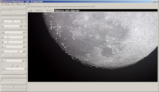
After setting the sliders for "Smoothing Factor" (to handle noise), "Minimum Distance" (to determine how many reference points will be used - the larger the minimum distance the fewer reference points), "Search Radius" (how many pixels over to scan, at most, to find the reference point in the next frame), "Correlation Area Radius (how large an area to process to correlate the feature of interest), and the "Frame Extension" (to determine how close to the edge of the frame to still process reference points), when you hit "Set R Points" AviStack will generate the entire set of reference points that it will attempt to match for stacking. (Figure 15)

Figure 15 - Reference Points are Set.

You can fine-tune the placement of reference points by removing points (click within 5 pixels of an existing point and it will be removed, or remove a rectangular area of points by right clicking and dragging a rectangle) or adding points (by clicking the place where you want the new point to  go).  It makes sense to have fewer points in regions that are relatively "flat" and do not have features, and perhaps to place more reference points where there is a lot of fine detail in the image.

This is a great time to save the AviStack Data file, to capture the work that you have done so far. .If you have .asd files saved at this step - after you have "Set R Points" - you can later reload these files for batch processing.  If you have several image sets in your project, batch processing is highly recommended!  You can run the batch overnight (it might actually take that long!) rather than watching AviStack as it executes the time consuming steps of "Calculate Quality", "Align Reference Points", and "Stack Frames".  It is much more productive to take all of your image sets past to the "Set R Points" step, and then process all of them as .asd files loaded into a batch, instead of sitting there while AviStack processes the data for tens of minutes (or hours!)

The Calculate Quality step is used to limit the frames that will be stacked to just those that have the quality higher than the Quality Cutoff that you set with the associated slider.  A quality cutoff of 30% means that only the best 30% of the frames will be stacked. The Quality Area Size slider is used to set the size of rectangles that will be used to evaluate the quality - the smaller the area the larger the number of individual rectangles, each of which will be evaluated for quality. (Figure 16)  I have not been able to find a technical description of what is meant by the term "quality" in this step.  However, it seems to be related to the size of features resolved (smaller is better) and the sharpness of the edges (sharper is better).

Figure 16 - Calculating the Quality of the area inside of each rectangle.

When the quality calculation is completed, a graph of the average frame quality is presented. (Figure 17)  In this graph, the average quality of the frame, apparently calculated as the average of all of the individual quality rectangles on that frame, is reported as being better or worse than the reference frame.  If we could, we might want to only stack images that were better than our reference frame (i.e. greater than 0.0 quality).

 

Figure 17 - Average Frame Quality.

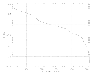
If we open the Diagram for Quality (Sorted) we are presented with the following graph (Figure 18):

 

Figure 18 - Frames Sorted by Quality.

From this graph we can see that if we wanted to only stack images that had an average quality at least 10% better than our reference image, we would still have more than 100 images to stack.  One way we could actually do this is tosave out the frames using the Films, Quality Sorted > TIFF into a directory, and then reload the project using File, Load Folder.  Naturally, image 1.tiff would be our reference image (since it has the highest quality rating), and we would choose to process only images 1.tiff to 100.tiff from that directory.

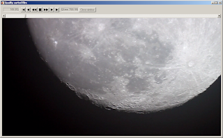
To get a visual idea of what the frames look like, in order of quality, we can use the Films, Quality Sorted menu to open a window where we can step through the frames in sorted order.  The frame number that is being shown is the current frame; you will notice that the number jumps around as it navigates to the next best image.  Also, there is a QArea number that presents a numerical value for the quality of the current rectangle area under the cursor (although the rectangle is not shown), so you can get an idea of the quality value that has been calculated for that area. (Figure 19)

 

Figure 19 - The Quality Sorted Film Reviewer.

Once we have calculated the quality, and set the quality cutoff, then we are ready to go to the "Align Reference Points" stage.  This is were the main processing of AviStack gets done.  The program inspects every reference point, in all of the frames, and accepts or rejects the point for stacking based on the parameters set by the quality cutoff.  You might think that it will only do this for the number of frames that fall within the quality cutoff that you have set in the previous stage.  However, if you watch the graphical display as it performs this task you will see that performs the calculation for all frames that were not excluded in the Align Frames step.  (For example, in my test I used a quality cutoff of 5% and AviStack reported that 26 frames would be processed.  However, I watched 323 frames being processed - the number set in the Align Frames step.)  I can only suggest that perhaps the quality cutoff relates to the quality of the rectangular quality areas, rather than the frames, and that it stacks any reference point in the quality area that exceeds the quality threshold in each frame.  (None of the documentation that I can find is clear about this.  You can watch the process for yourself and decide...)  As it processes each frame some reference points are rendered as white crosses; and some are black crosses.  White crosses are reference points that will be used for stacking; black crosses are rejected reference points. (Figure 20)

Figure 20 - Aligning Reference Points.

When the aligning process is completed a histogram is presented to show the distribution of deviations (in pixels) for the reference points that have been aligned. (Figure 21)

Figure 20 - The reference Point Distribution.

Note that this histogram has a log scale, so the distribution is heavily in favor of 0-1 pixels (which is what we want!)

Finally we are ready to Stack Frames!  There is a radio button choice to "Crop" or "Original Size".  If the resulting image is going to be stitched to other images to make a mosaic this should be set to :"Crop", to that the edges that may not have been aligned are not used to try to match regions on adjoining images.  In the stacking process the small regions around the reference points are rendered, frame by frame, against the background, or averaged with the stacked pieces that are already there, to ultimately render the entire image. (Figure 21)

 

Figure 21 - Frame Stacking in Progress.

The output of the stacking process is the finished frame, which can be saved as a .fits or .tiff file.  If you are making a mosaic, or if you want to compare images constructed from different sequences, you should also

save your settings, or set them as default, so that you can use the same parameters for processing the other image sets.  So after all of that, here is the final image (Figure 22)

 

Figure 22 - The Final Stacked Image.

OK, I cheated.  This is actually the image created by stacking the best 10 tiff images from the directory of .individual frames created by the Films, Quality Sorted > TIFF command.  You can compare this with Figure 5, which was the real output from stacking 326 frames with a quality cutoff of 30%.  I will let you judge for yourself which image is better...

The last option is to play with the experimental wavelet sharpening option, but that is a task for another day.